Python 语言清理时间序列数据

欢迎，来自IP地址为：216.73.216.58 的朋友

---

在 现实世界是，时间序列数据很少是干净的。传感器会掉线，系统时钟会漂移，管道会造成重复记录，手动录入数据也会引入错误。当数据集到达处理端时，它已经经历了采集、传输和存储，每一步都可能造成数据损坏。

清洗时间序列数据比清洗表格数据更难，因为时间是一个结构约束，我们不能随意打乱行顺序，也不能用列均值来填补缺失值，否则就会把未来的数据混入过去的观测值中。每一个清洗决策都必须尊重时间顺序，否则就会破坏基时序所构建的所有数据的完整性。

本文将逐步介绍 Python 语言实现的完整清洗流程：从原始数据到生成可用于特征工程或建模的数据集。我们将涵盖缺失值检测和填补、异常值识别和处理、重复值处理、频率对齐、噪声平滑和模式验证，并在整个过程中应用于示例传感器数据。

系统需求

要学习本教程，可能需要如下技能：

• 熟练使用 Python 和 pandas DataFrame
• 熟悉时间索引数据
• 了解特征工程和机器学习建模的基本原理

我们将使用 pandas 和 numpy 进行数据处理，使用 scipy 进行信号平滑和统计检验，使用 scikit-learn 进行异常检测，并使用 statsmodels 进行季节性分解。在运行本教程中的任何代码之前，需要安装这些库：

pip install pandas numpy scipy scikit-learn statsmodels

如何审核时间序列

数据清洗的第一条原则是：先检查再删除。在进行插补、平滑或删除任何数据之前，都需要全面了解问题所在。

一次全面的审核应涵盖以下内容：

• 时间索引：是否规律？是否存在时间缺失？
• 缺失值分布：缺失值是随机分布还是聚集分布？
• 值范围：是否存在明显的缺失值或传感器故障？
• 重复的时间戳

我们首先创建一个示例数据集（包含上述部分问题）：

import pandas as pd
import numpy as np

# Simulate one week of smart grid voltage readings (hourly)
# with realistic problems injected
periods = 168
index = pd.date_range("2026-06-01", periods=periods, freq='h')

voltage = (
        220.0
        + 3.5 * np.sin(2 * np.pi * np.arange(periods) / 24)
        + np.random.normal(0, 1.2, periods)
)

# Inject problems
voltage[14:17] = np.nan          # sensor dropout: 3 consecutive missing
voltage[42] = np.nan             # isolated missing
voltage[78] = 312.4              # spike outlier
voltage[101:104] = np.nan        # another dropout
voltage[130] = 187.2             # dip outlier

series = pd.Series(voltage, index=index, name="voltage_v")

# --- Audit ---
print("=== TIME SERIES AUDIT ===")
print(f"Period:        {series.index.min()} → {series.index.max()}")
print(f"Observations:  {len(series)}")
print(f"Expected freq: {pd.infer_freq(series.index)}")
print(f"\nMissing values: {series.isna().sum()} ({series.isna().mean()*100:.1f}%)")
print(f"Value range:    [{series.min():.2f}, {series.max():.2f}]")
print(f"Mean ± Std:     {series.mean():.2f} ± {series.std():.2f}")

# Identify consecutive missing runs
missing_mask = series.isna()
missing_runs = []
run_start = None
for i, (ts, is_missing) in enumerate(missing_mask.items()):
    if is_missing and run_start is None:
        run_start = ts
    elif not is_missing and run_start is not None:
        missing_runs.append((run_start, missing_mask.index[i - 1]))
        run_start = None

print(f"\nMissing runs ({len(missing_runs)} total):")
for start, end in missing_runs:
    print(f"  {start} → {end}")

输出为：

本次审计为我们在开始数据清洗之前，提供了一份关于数据损坏状况的”地图”。其核心任务在于区分两类缺失值：一类是孤立的缺失值，可通过局部上下文进行填补；另一类是连续大段的缺失值，这类情况可能需要采取不同的处理策略，或需加以标记以提示数据使用者。

如何重采样至标准频率

在填补缺失值之前，我们需要确认所使用的时间索引实际上是规律的。在已导入的时间序列数据中，一个常见的问题是：缺失的时间戳往往是直接”缺席”了，而非以 NaN 行的形式呈现–这意味着调用”.fillna()”方法将无法识别并处理这些缺失值。

import pandas as pd
import numpy as np

# Simulate one week of smart grid voltage readings (hourly)
# with realistic problems injected
periods = 168
index = pd.date_range("2026-06-01", periods=periods, freq='h')

voltage = (
        220.0
        + 3.5 * np.sin(2 * np.pi * np.arange(periods) / 24)
        + np.random.normal(0, 1.2, periods)
)

# Inject problems
voltage[14:17] = np.nan          # sensor dropout: 3 consecutive missing
voltage[42] = np.nan             # isolated missing
voltage[78] = 312.4              # spike outlier
voltage[101:104] = np.nan        # another dropout
voltage[130] = 187.2             # dip outlier

series = pd.Series(voltage, index=index, name="voltage_v")

# Simulate a sensor feed with missing timestamps (not just missing values)
irregular_index = index.delete([14, 15, 16, 42, 101, 102, 103])
irregular_series = series.dropna().reindex(irregular_index)

print(f"Original length:   {len(series)}")
print(f"Irregular length:  {len(irregular_series)}")
print(f"Inferred freq:     {pd.infer_freq(irregular_series.index)}")  # None = irregular

# Reindex to the full canonical hourly grid
canonical_index = pd.date_range(
    start=irregular_series.index.min(),
    end=irregular_series.index.max(),
    freq="h"
)

reindexed = irregular_series.reindex(canonical_index)

print(f"\nAfter reindex:")
print(f"Length:         {len(reindexed)}")
print(f"Missing values: {reindexed.isna().sum()}")
print(f"Inferred freq:  {pd.infer_freq(reindexed.index)}")

输出如下：

“pd.infer_freq”函数返回”None”则表示索引存在缺失值。重新索引到规范网格后，缺失的时间戳会明确地显示为”NaN”行，此时我们的插补逻辑就可以找到它们了。

如何处理缺失值

并非所有缺失值都需要采用相同的处理方式。对于平滑信号中单个孤立的缺失值，最好使用插值法进行填充。然而，对于波动较大的信号，例如传感器出现 3 小时的数据丢失，则最好标记出来而不是伪造缺失值。处理策略应同时考虑数据缺失的长度和信号的特性。

前向填充–适用于阶跃函数信号

当变量保持其最后已知值直至发生改变时（例如机器状态、设定值或类别标志），前向填充是合适的。

import pandas as pd
import numpy as np

# Simulate one week of smart grid voltage readings (hourly)
# with realistic problems injected
periods = 168
index = pd.date_range("2026-06-01", periods=periods, freq='h')

voltage = (
        220.0
        + 3.5 * np.sin(2 * np.pi * np.arange(periods) / 24)
        + np.random.normal(0, 1.2, periods)
)

# Inject problems
voltage[14:17] = np.nan          # sensor dropout: 3 consecutive missing
voltage[42] = np.nan             # isolated missing
voltage[78] = 312.4              # spike outlier
voltage[101:104] = np.nan        # another dropout
voltage[130] = 187.2             # dip outlier

series = pd.Series(voltage, index=index, name="voltage_v")

# Equipment operating mode — a step signal
mode_data = pd.Series(
    ["running", "running", np.nan, np.nan, "idle", "idle", np.nan, "running"],
    index=pd.date_range("2026-06-01", periods=8, freq="h"),
    name="operating_mode"
)

filled_mode = mode_data.ffill()
print(pd.DataFrame({"original": mode_data, "ffill": filled_mode}))

输出结果为：

时间加权插值–适用于连续信号

对于连续的传感器读数，时间加权线性插值能够正确处理不规则的间断，因为它不假设间隔相等。

import pandas as pd
import numpy as np

# Simulate one week of smart grid voltage readings (hourly)
# with realistic problems injected
periods = 168
index = pd.date_range("2026-06-01", periods=periods, freq='h')

voltage = (
        220.0
        + 3.5 * np.sin(2 * np.pi * np.arange(periods) / 24)
        + np.random.normal(0, 1.2, periods)
)

# Inject problems
voltage[14:17] = np.nan          # sensor dropout: 3 consecutive missing
voltage[42] = np.nan             # isolated missing
voltage[78] = 312.4              # spike outlier
voltage[101:104] = np.nan        # another dropout
voltage[130] = 187.2             # dip outlier

series = pd.Series(voltage, index=index, name="voltage_v")

irregular_index = index.delete([14, 15, 16, 42, 101, 102, 103])
irregular_series = series.dropna().reindex(irregular_index)

# Reindex to the full canonical hourly grid
canonical_index = pd.date_range(
    start=irregular_series.index.min(),
    end=irregular_series.index.max(),
    freq="h"
)

reindexed = irregular_series.reindex(canonical_index)

# Fill the voltage series using time-based interpolation
voltage_clean = reindexed.interpolate(method="time")

# Compare original vs filled around the first gap
gap_window = voltage_clean["2026-06-01 12:00":"2026-06-01 18:00"]
original_window = reindexed["2026-06-01 12:00":"2026-06-01 18:00"]

comparison = pd.DataFrame({
    "original":     original_window,
    "interpolated": gap_window.round(3),
    "was_missing":  original_window.isna(),
})
print(comparison)

输出是：

周期性分解插补–针对较长的缺失值

对于周期性信号中超过几个周期的缺失值，直接插值会忽略周期性模式。更好的方法是分解序列，分别对每个分量进行插补，然后再进行重构。

import pandas as pd
import numpy as np
from statsmodels.tsa.seasonal import seasonal_decompose

# Use a longer series for decomposition (needs enough periods)
long_voltage = pd.Series(
    220.0
    + 3.5 * np.sin(2 * np.pi * np.arange(336) / 24)
    + np.random.normal(0, 1.0, 336),
    index=pd.date_range("2026-06-01", periods=336, freq="h")
)

# Inject a 6-hour gap
long_voltage.iloc[100:106] = np.nan

# Interpolate first to give decompose a complete series to work with
temp_filled = long_voltage.interpolate(method="time")
decomp = seasonal_decompose(temp_filled, model="additive", period=24)

# Reconstruct: trend + seasonal + zero residual for missing positions
reconstructed = long_voltage.copy()
missing_idx = long_voltage[long_voltage.isna()].index
reconstructed[missing_idx] = (
        decomp.trend[missing_idx].ffill()
        + decomp.seasonal[missing_idx]
)

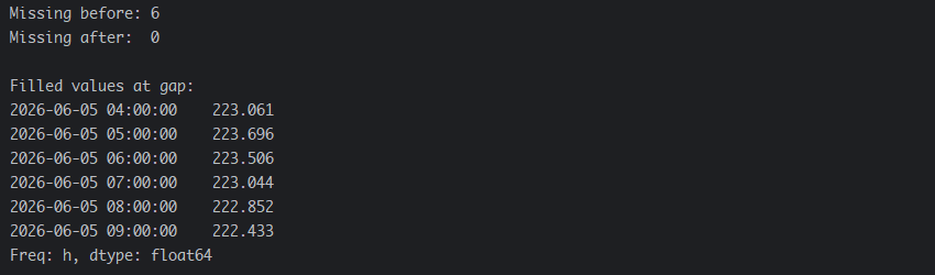
print(f"Missing before: {long_voltage.isna().sum()}")
print(f"Missing after:  {reconstructed.isna().sum()}")
print("\nFilled values at gap:")
print(reconstructed[missing_idx].round(3))

季节分解插补法兼顾了日内时间模式，正如以下结果所见，填补后的数值并非在缺失处呈现为一条直线，而是遵循了预期的日内曲线走势。

如何检测与处理异常值

相比于表格数据，时间序列中的异常值处理起来更为棘手，因为其所处的”上下文”至关重要。例如，电压出现异常的高峰或低谷，既可能仅仅是传感器产生的瞬时尖峰信号，也可能是电网中确实发生的重大事件。因此，就需要采用那些能够利用时间上下文信息、而非仅仅依赖全局统计数据的检测方法。

基于滚动窗口的 Z-Score 方法

单纯使用全局 Z-Score 方法，往往会遗漏非平稳时间序列中的局部异常。相比之下，滚动 Z-Score 方法能够识别出那些相对于其局部邻域而言显得异常的数值。

注：非平稳时间序列是指那些统计特性（如均值、方差或趋势）随时间推移而发生变化、而非保持恒定的时间序列。

import pandas as pd
import numpy as np

# Simulate one week of smart grid voltage readings (hourly)
# with realistic problems injected
periods = 168
index = pd.date_range("2026-06-01", periods=periods, freq='h')

voltage = (
        220.0
        + 3.5 * np.sin(2 * np.pi * np.arange(periods) / 24)
        + np.random.normal(0, 1.2, periods)
)

# Inject problems
voltage[14:17] = np.nan          # sensor dropout: 3 consecutive missing
voltage[42] = np.nan             # isolated missing
voltage[78] = 312.4              # spike outlier
voltage[101:104] = np.nan        # another dropout
voltage[130] = 187.2             # dip outlier

series = pd.Series(voltage, index=index, name="voltage_v")

irregular_index = index.delete([14, 15, 16, 42, 101, 102, 103])
irregular_series = series.dropna().reindex(irregular_index)

# Reindex to the full canonical hourly grid
canonical_index = pd.date_range(
    start=irregular_series.index.min(),
    end=irregular_series.index.max(),
    freq="h"
)

reindexed = irregular_series.reindex(canonical_index)

# Fill the voltage series using time-based interpolation
voltage_clean = reindexed.interpolate(method="time")

window = 24  # 24-hour rolling window

roll_mean = voltage_clean.rolling(window, center=True, min_periods=1).mean()
roll_std  = voltage_clean.rolling(window, center=True, min_periods=1).std()

rolling_z = (voltage_clean - roll_mean) / roll_std

threshold = 3.0
outliers_z = rolling_z[rolling_z.abs() > threshold]

print(f"Rolling Z-score outliers detected: {len(outliers_z)}")
print(outliers_z.round(3))

输出是：

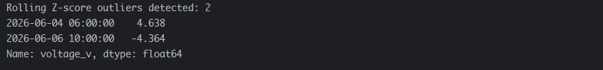
Z-score 异常值检测对于近似高斯（正态）分布的数据效果最佳，因为它假定数据以均值为中心，并呈现出由标准差衡量的对称分布。

基于 IQR 的异常值检测

对于检测非高斯分布中的异常值，四分位距（IQR）方法具有更强的适应性。四分位距（IQR）是指第三四分位数（Q3）与第一四分位数（Q1）之差，它代表了数据中间 50% 部分的离散程度。

import pandas as pd
import numpy as np

# Simulate one week of smart grid voltage readings (hourly)
# with realistic problems injected
periods = 168
index = pd.date_range("2026-06-01", periods=periods, freq='h')

voltage = (
        220.0
        + 3.5 * np.sin(2 * np.pi * np.arange(periods) / 24)
        + np.random.normal(0, 1.2, periods)
)

# Inject problems
voltage[14:17] = np.nan          # sensor dropout: 3 consecutive missing
voltage[42] = np.nan             # isolated missing
voltage[78] = 312.4              # spike outlier
voltage[101:104] = np.nan        # another dropout
voltage[130] = 187.2             # dip outlier

series = pd.Series(voltage, index=index, name="voltage_v")

irregular_index = index.delete([14, 15, 16, 42, 101, 102, 103])
irregular_series = series.dropna().reindex(irregular_index)

# Reindex to the full canonical hourly grid
canonical_index = pd.date_range(
    start=irregular_series.index.min(),
    end=irregular_series.index.max(),
    freq="h"
)

reindexed = irregular_series.reindex(canonical_index)

# Fill the voltage series using time-based interpolation
voltage_clean = reindexed.interpolate(method="time")

Q1 = voltage_clean.quantile(0.25)
Q3 = voltage_clean.quantile(0.75)
IQR = Q3 - Q1

lower_bound = Q1 - 1.5 * IQR
upper_bound = Q3 + 1.5 * IQR

outliers_iqr = voltage_clean[
    (voltage_clean < lower_bound) | (voltage_clean > upper_bound)
    ]

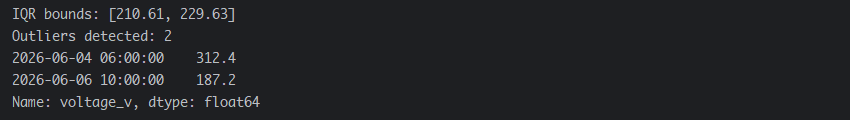
print(f"IQR bounds: [{lower_bound:.2f}, {upper_bound:.2f}]")
print(f"Outliers detected: {len(outliers_iqr)}")
print(outliers_iqr.round(2))

输出结果为：

隔离森林算法–用于多变量异常值检测

如果拥有多个传感器时，虽然单个通道的读数可能看起来正常，但将其与其他通道的读数结合起来，就能发现异常。隔离森林算法能够自然地处理这种情况。

import pandas as pd
import numpy as np
from sklearn.ensemble import IsolationForest

n = 200

sensor_df = pd.DataFrame({
    "voltage_v":    220 + 3 * np.sin(2 * np.pi * np.arange(n) / 24) + np.random.normal(0, 1, n),
    "current_a":    15  + 0.8 * np.sin(2 * np.pi * np.arange(n) / 24) + np.random.normal(0, 0.3, n),
    "frequency_hz": 50  + np.random.normal(0, 0.05, n),
}, index=pd.date_range("2026-06-01", periods=n, freq="h"))

# Inject a multivariate anomaly — voltage drops, current spikes together
sensor_df.iloc[88, 0] = 194.2   # voltage dip
sensor_df.iloc[88, 1] = 28.7    # current surge (consistent with fault)

clf = IsolationForest(contamination=0.02, random_state=42)
sensor_df["anomaly_score"] = clf.fit_predict(sensor_df[["voltage_v", "current_a", "frequency_hz"]])

anomalies = sensor_df[sensor_df["anomaly_score"] == -1]
print(f"Anomalies detected: {len(anomalies)}")
print(anomalies[["voltage_v", "current_a", "frequency_hz"]].round(2))

输出如下图所示：

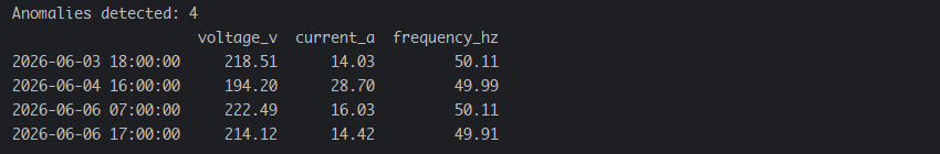
在实际使用时，我们就可以利用特定领域的阈值规则来对异常分数进行后续处理。

异常值处理

一旦识别出异常值，就可以采用以下几种方式进行处理：

• 利用 Winsorization 方法对其进行封顶处理，即将极端值限制在某一阈值范围内
• 将其替换为插值或估算值
• 对其进行标记，以便模型能够进行恰当的处理

示例代码如下：

import pandas as pd
import numpy as np

# Simulate one week of smart grid voltage readings (hourly)
# with realistic problems injected
periods = 168
index = pd.date_range("2026-06-01", periods=periods, freq='h')

voltage = (
        220.0
        + 3.5 * np.sin(2 * np.pi * np.arange(periods) / 24)
        + np.random.normal(0, 1.2, periods)
)

# Inject problems
voltage[14:17] = np.nan          # sensor dropout: 3 consecutive missing
voltage[42] = np.nan             # isolated missing
voltage[78] = 312.4              # spike outlier
voltage[101:104] = np.nan        # another dropout
voltage[130] = 187.2             # dip outlier

series = pd.Series(voltage, index=index, name="voltage_v")

irregular_index = index.delete([14, 15, 16, 42, 101, 102, 103])
irregular_series = series.dropna().reindex(irregular_index)

# Reindex to the full canonical hourly grid
canonical_index = pd.date_range(
    start=irregular_series.index.min(),
    end=irregular_series.index.max(),
    freq="h"
)

reindexed = irregular_series.reindex(canonical_index)

# Fill the voltage series using time-based interpolation
voltage_clean = reindexed.interpolate(method="time")

Q1 = voltage_clean.quantile(0.25)
Q3 = voltage_clean.quantile(0.75)
IQR = Q3 - Q1

lower_bound = Q1 - 1.5 * IQR
upper_bound = Q3 + 1.5 * IQR

outliers_iqr = voltage_clean[
    (voltage_clean < lower_bound) | (voltage_clean > upper_bound)
    ]

# Winsorize: cap at the IQR bounds
voltage_winsorized = voltage_clean.clip(lower=lower_bound, upper=upper_bound)

# Replace outliers with time-interpolated values
voltage_outlier_fixed = voltage_clean.copy()
voltage_outlier_fixed[outliers_iqr.index] = np.nan
voltage_outlier_fixed = voltage_outlier_fixed.interpolate(method="time")

print("Outlier treatment comparison:")
for ts in outliers_iqr.index:
    print(f"\n  {ts}")
    print(f"    Original:     {voltage_clean[ts]:.2f}")
    print(f"    Winsorized:   {voltage_winsorized[ts]:.2f}")
    print(f"    Interpolated: {voltage_outlier_fixed[ts]:.2f}")

输出：

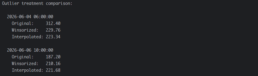
温莎化处理保留了数据点本身，但将其截断至一个合理的取值范围内–如果希望保留”发生了异常情况”这一信息时，这种方法非常有用。插值法则将离群值视为缺失数据进行处理–如果认为该读数纯属错误时，这种方法更为适宜。

如何移除重复项

当数据通道在发生故障后进行重试时，重复的时间戳是常见的现象。与表格数据中的重复项不同，时间序列数据中的重复项并非总是完全一致的；在重试过程中，针对同一时间戳所获取的读数可能会略有差异。

import pandas as pd
import numpy as np

# Simulate one week of smart grid voltage readings (hourly)
# with realistic problems injected
periods = 168
index = pd.date_range("2026-06-01", periods=periods, freq='h')

voltage = (
        220.0
        + 3.5 * np.sin(2 * np.pi * np.arange(periods) / 24)
        + np.random.normal(0, 1.2, periods)
)

# Inject problems
voltage[14:17] = np.nan          # sensor dropout: 3 consecutive missing
voltage[42] = np.nan             # isolated missing
voltage[78] = 312.4              # spike outlier
voltage[101:104] = np.nan        # another dropout
voltage[130] = 187.2             # dip outlier

series = pd.Series(voltage, index=index, name="voltage_v")

irregular_index = index.delete([14, 15, 16, 42, 101, 102, 103])
irregular_series = series.dropna().reindex(irregular_index)

# Reindex to the full canonical hourly grid
canonical_index = pd.date_range(
    start=irregular_series.index.min(),
    end=irregular_series.index.max(),
    freq="h"
)

reindexed = irregular_series.reindex(canonical_index)

# Fill the voltage series using time-based interpolation
voltage_clean = reindexed.interpolate(method="time")

Q1 = voltage_clean.quantile(0.25)
Q3 = voltage_clean.quantile(0.75)
IQR = Q3 - Q1

lower_bound = Q1 - 1.5 * IQR
upper_bound = Q3 + 1.5 * IQR

outliers_iqr = voltage_clean[
    (voltage_clean < lower_bound) | (voltage_clean > upper_bound)
    ]

# Winsorize: cap at the IQR bounds
voltage_winsorized = voltage_clean.clip(lower=lower_bound, upper=upper_bound)

# Replace outliers with time-interpolated values
voltage_outlier_fixed = voltage_clean.copy()
voltage_outlier_fixed[outliers_iqr.index] = np.nan
voltage_outlier_fixed = voltage_outlier_fixed.interpolate(method="time")

# Inject duplicate timestamps with slightly different values (retry scenario)
dup_index = index.tolist()
dup_index.insert(20, index[20])  # exact duplicate timestamp
dup_index.insert(55, index[55])  # retry duplicate

dup_values = voltage_clean.tolist()
dup_values.insert(20, voltage_clean.iloc[20])
dup_values.insert(55, voltage_clean.iloc[55] + 0.7)  # slightly different value

dup_series = pd.Series(dup_values, index=pd.DatetimeIndex(dup_index), name="voltage_v")

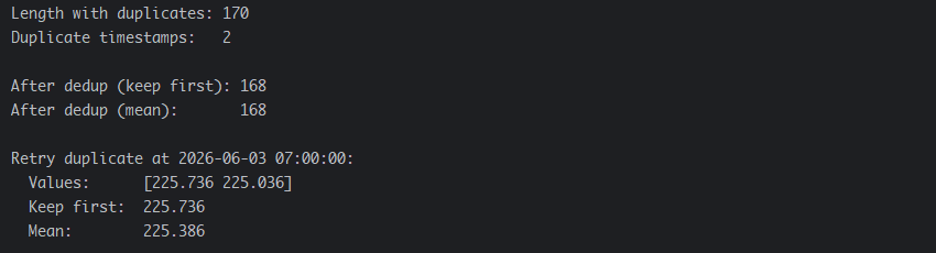
print(f"Length with duplicates: {len(dup_series)}")
print(f"Duplicate timestamps:   {dup_series.index.duplicated().sum()}")

# Strategy 1: keep first (original reading)
dedup_first = dup_series[~dup_series.index.duplicated(keep="first")]

# Strategy 2: keep mean (average across retries)
dedup_mean = dup_series.groupby(level=0).mean()

print(f"\nAfter dedup (keep first): {len(dedup_first)}")
print(f"After dedup (mean):       {len(dedup_mean)}")

# Show the retry duplicate
ts_retry = index[55]
print(f"\nRetry duplicate at {ts_retry}:")
print(f"  Values:      {dup_series[ts_retry].values.round(3)}")
print(f"  Keep first:  {dedup_first[ts_retry]:.3f}")
print(f"  Mean:        {dedup_mean[ts_retry]:.3f}")

执行结果如下：

频率对齐与重采样

实际的数据管道往往包含频率各异的数据。例如，可能需要将每分钟的仪表读数与每小时的天气数据流进行合并。在执行合并操作之前，就必须明确地对这些数据的频率进行对齐。

import pandas as pd
import numpy as np

power_1min = pd.Series(
    42 + 18 * ((pd.date_range("2026-06-01", periods=1440, freq="min").hour.isin(range(8, 19)))).astype(int)
    + np.random.normal(0, 2, 1440),
    index=pd.date_range("2026-06-01", periods=1440, freq="min"),
    name="power_kw"
)

# Downsample to hourly: mean is appropriate for power (average over the hour)
power_hourly_mean = power_1min.resample("h").mean().round(2)

# Downsample to hourly: max (peak demand within the hour)
power_hourly_max = power_1min.resample("h").max().round(2)

# Downsample to hourly: sum (total energy = kWh)
energy_hourly_kwh = (power_1min.resample("h").sum() / 60).round(3)

comparison = pd.DataFrame({
    "mean_kw":    power_hourly_mean,
    "peak_kw":    power_hourly_max,
    "energy_kwh": energy_hourly_kwh,
}).iloc[7:13]

print(comparison)

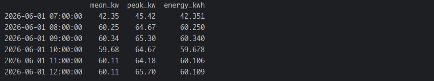
选择哪种聚合方式，对于下游应用而言至关重要。平均功率适用于负荷画像；峰值功率适用于容量规划；而求和（并转换为 kWh）则适用于计费。所谓的”正确答案”往往取决于具体的应用领域，而非单纯的技术考量。

总之，操作顺序至关重要。请先进行重索引，再执行缺失值填补；先填补缺失值，再进行平滑处理；待所有步骤完成后，最后进行验证。若跳过某些步骤或打乱操作顺序，由此累积的误差往往会相互叠加；一旦进入模型预测阶段，想要回溯并定位这些误差将变得极其困难。

时间序列数据的清洗工作或许并不光鲜亮丽，但相比于那些基于清洗不当的数据训练出的、哪怕再复杂的模型，一个基于干净数据和精心构建的特征训练出的模型，几乎总能取得更优异的表现。在对时间序列数据运行哪怕是最简单的算法之前，确保这一整套数据处理流程（Pipeline）的正确性，无疑是我们所能采取的、最具杠杆效应（即投入产出比最高）的关键举措。